Conversion Rate A B Testing

05 Jan 2022

Testing conversion rate improvements

Many internet companies use A/B testing to evaluate the performance of website changes they want to make. A typical metric in such scenarios is the conversion rate (CVR) of a user, i.e. the probability that a user converts (e.g. makes a purchase) on the website. A typical A/B test setup in such a situation would randomize users into two (equally sized) groups: the test group that would be exposed to the new experience and the control group that would be exposed to the status quo version of the website.

An analyst would do a power calculation based on the expected effect size from the test, the variation of the CVR metric, the desired type I and type II error bounds in order to determine the duration of the test. After the test the analyst might perform Fisher's exact test to determine whether or not to accept the new website version.

Larry's analysis

Let us consider the following fictitious example in which Larry the analyst of the internet company Nozama runs a 1-week-long A/B test. His data shows the following

	control	test
users	35000	35000
conversions	1394	1666

Larry uses python to compute the p-value of the Fisher exact statistic

from scipy import stats

data = [[1394, 1666], [35000 - 1394, 35000 - 1666]]
pval = stats.fisher_exact(data)[1]
print(pval)

The result is 5.4e-07 which is "statistically significant" w.r.t. to Larry's predefined 5% significance level.

Larry can't believe it, the new version improved the user conversion by 19.5%!

But has it really ?

Larry just blindly applied some statistical test to his data without thinking about the data generating process.

So what exactly are the assumptions that Larry implicitly used in his analysis ?

For the Fisher exact test we need to assume that we have independent, identically distributed conversion events. More precisely, we need to assume that (for each group) $Conversions \sim Bin(users, p)$ for some probability $p$, i.e. that the number of conversions in each group are drawn from a Binomial distribution with $n=$number of users and some fixed probability $p$ (the conversion rate).

A smarter approach

Using domain knowledge about how people on the website behave we know users that land on the website don't all necessarily convert on the same day but sometimes purchase with some time lag after the initial visit. With this knowledge at hand we take a new (Bayesian) approach to analysing the test results.

We make the following model assumptions:

$p$ = probability of conversion
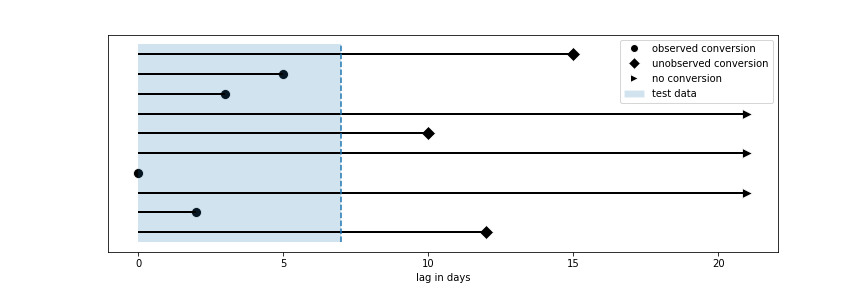
$X$ = lag in days between user website visit and conversion, where $X=\infty$ corresponds to no conversion
Conditional on a conversion, we assume that the lag variable $X$ is distributed according to a zero-inflated geometric distribution.

We can write the pmf and cdf (for $k<\infty$) of $X$ as follows:

\[P(X=k) = (1-p)\cdot \mathbb{1}_{\{\infty\}}(k) + p\cdot (\pi\cdot \mathbb{1}_{\{0\}}(k) + (1-\pi)\cdot\lambda \cdot(1-\lambda)^k\cdot \mathbb{1}_{\{\geq 0\}}(k))\] \[F(k) = P(X \leq k) = p(1 -(1-\pi)(1-\lambda)^{k+1}).\]

Before we can fit the model to our data there is one more problem that we encounter. Users in our data set for which we didn't observe a conversion could either be truly non-converting or we haven't been able to observe their conversion yet, since we are only considering 1 week of data. Users that entered our experiment on the first day for which we haven't observed a conversion will have a smaller probability to still convert since we know that they didn't do a purchase in one of the following 6 days. On other other hand, users that entered our experiment on the 7th day will have a relatively larger probability to still convert on one of the following days. We are faced with a so called censored data problem.

A subsample of our data looks as follows:

visit_date	conversion_date	users	is_control
2021-12-01	2021-12-01	84	1
2021-12-01	None	4750	1
2021-12-02	2021-12-04	33	1
2021-12-02	None	4785	1
2021-12-01	2021-12-05	2	0
2021-12-01	None	4756	0
2021-12-02	2021-12-02	199	0
2021-12-02	None	4762	0

visualization of censored data

We can write a Stan program in order to fit a model on the test and control data separately. We use Stan's custom distribution functions capability (see here for a tutorial) to code the pmf, cdf, inverse cdf and ccdf of our model as follows:

functions{
    real uncensored_lpmf(int y, real pi, real p, real lambda){
        if (y == 0) 
            return log(p) + log(pi + (1 - pi) * lambda);
        else
            return log(p) + log(1 - pi) + log(lambda) + y * log(1 - lambda);
        }

    real censoredccdf(real y, real pi, real p, real lambda){
        return log(1 - p + p * (1 - pi) * pow(1 - lambda, y + 1));
        }
        
     real invcdf(real u, real pi, real p, real lambda){
         if (u > p)
             return -1;
         else
             return ceil(log( (p - u) / (p * (1 - pi)) ) / log(1 - lambda) - 1);
     }
    
     real uncensored_rng(real pi, real p, real lambda) {
         real u;
         u = uniform_rng(0, 1);
         return invcdf(u, pi, p, lambda);
     }
}

Because we know that the typical conversion rate of our website is around 5% and unlikely to be larger than 10% we put a $Beta(2, 38)$-prior on the $p$-parameter. We also know that there are disproportionally many users that convert on the day of their first visit which is why we assume a non-negative value of $\pi$ but with slightly more weight towards $0$ which leads us to specify the prior $\pi\sim Beta(1,2)$. Finally, we put a non-informative uniform prior on the "success"-probability $\lambda$. Note, that values $\max\{-1, \frac{-(1-\lambda)}{\lambda}\} \leq \pi < 1$ would still give a well-defined model, and would allow for a zero-deflated geometric distribution as well.

You can find our complete Stan model here.

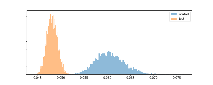
Fitting the model to the data above we obtain the following posterior distributions for $p$ for the test and control groups, respectively.

posterior distribution of $$p$$ posterior distribution of $p$

As we can clearly see from the plot we are almost 100% certain (given the model and the data) that our control version has a higher conversion rate $p$ than the new test variant. So we should definitively not accept the new website variant.

How is this possible ?

By inspecting all the posterior parameters of the model (not just the conversion rate $p$) we see that the new website increased the parameters $\pi$ and $\lambda$ of our zero-inflated geometric distribution of the time-to-conversion (aka lag) variable $X$, i.e. although users convert less frequently under the new website version, the ones that do, do so with a smaller time lag from their initial website visit.

Looking at what the new website version does, this seems plausible: the new website version implemented urgency features that gave the users the impression that the product they were considering for purchase would soon be unavailable or would drastically increase in price. This lead to the fact that some users were annoyed by this alarmist messaging and design, and now didn't convert anymore even though they might have under the old version, and the ones that still did, now did so without letting too much time go by.

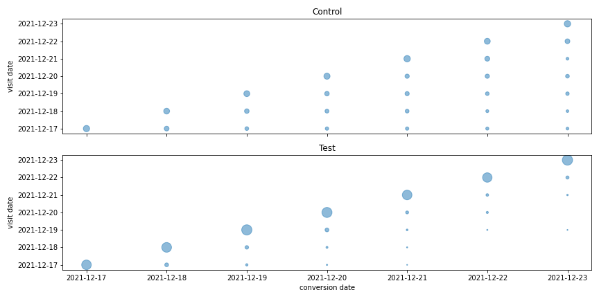visit vs. conversion date frequencies

Of course, at this point this can only be a hypothesis that is based on domain knowledge about how users typically react to certain changes and that fits with the data observed in this experiment. This cannot be so easily proven. A necessary condition for this explanation to be correct would be that we have treatment effect heterogeneity, i.e. that some users are affected differently by the change than others. We will leave a discussion about treatment effect heterogeneity for another blog post in the future.

Conclusions

Assumptions matter for correct decision making; think about the data generating process; domain knowledge is important
Be careful when using lagged response variables in A/B testing
Bayesian stats and Stan are awesome ;)

References / further reading

Our model was inspired by the continuous (frequentist) conversion model that was proposed in the 2014 KDD paper "Modeling delayed feedback in display advertising" by Olivier Chapelle.
Check out the Stan manual on estimating censored values.

Additions

20220109 - In response to some comments on Hacker News
Could Larry have just let the test run longer to make the correct decision ?

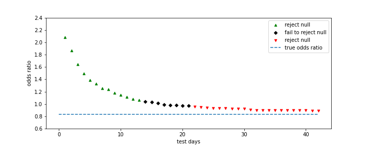
Letting the test run longer can be a method to avoid drawing wrong conclusions using the simpler approach of e.g. performing Fisher's exact test. The necessary test duration however, very much depends on the typical lag that is expected between visit and conversion (which can vary, e.g. by industry and also the attribution model used). It also depends on how strong the effect of the test is on the lag parameters $\pi$ and $\lambda$ vs. the effect on the conversion parameter $p$. For the simulated data set we can see how Larry's conclusion would have differed, had he run the test for different durations. Fisher's exact test results by test duration
Any test duration up to 13 days would have lead Larry to make the wrong conclusion about the test performance. For a test duration between 14 and 21 days Larry would have failed to reject the null hypothesis (at least not wrongfully accepting an inferior website version). Only for a test duration longer than 3 weeks would Larry have concluded that the test version actually performs worse than the control version (w.r.t. the CVR as KPI for the test). We can see that even after 6 weeks of testing the calculated odds ratio (i.e. the ratio of the conversion rates of both groups) is still almost 7% larger than the true odds ratio in this example.
In summary, letting the test run longer can be a solution to avoid more complicated stats in certain (many?) situations. An argument in favor of using the proposed conversion lag model is that it allows to reduce testing time while still coming to the correct conclusion.
Best is to use domain knowledge and business judgment to decide on how to best proceed in any given real-life situation.